Causal Inference: How to Move From Correlation to Cause

Causal inference is having a moment in the data industry, and it is not because the math is new. Rubin's potential outcomes framework dates to the 1970s. Judea Pearl's do-calculus is 30 years old. Difference-in-differences goes back to a cholera study in 1850s London.

What changed is the supply of data and the cost of analyzing it. Every company now sits on warehouses of behavioral, transactional, and conversational records, plus open-source libraries like DoWhy, EconML, and CausalML that put estimation and refutation methods within reach of any analytics team. The bottleneck moved from computation to interpretation.

And interpretation is where most analytics still breaks. Consider a real example from a public data report: across 8,504 Google reviews of Marriott-family hotels in Orlando, "front desk and check-in" was mentioned in 27.2% of comments, more than any other topic, and standard driver analysis flagged it as the number-two thing to fix. Run a formal causal model on the same reviews, controlling for property, tier, language, and review length, and the front desk has an effect of about two points on the odds of a one-star stay. Not statistically significant. Cleanliness, mentioned a third as often, causes a 34-point swing.

Same data, opposite instructions. So how do you tell which patterns in your data actually cause the outcome, and which ones are just riding along?

Key takeaway: Causal inference is the set of methods for estimating what would have happened under a different action, which is the only way to separate a driver from a coincidence and rank fixes by what they are actually worth.

What is causal inference?

Causal inference is the process of estimating the effect of a cause on an outcome from data. Not whether two things move together, but whether changing one would change the other, and by how much.

The distinction sounds academic until you have to spend a budget. A correlational finding tells you that accounts with frequent support contacts churn more often. A causal finding tells you that reducing repeat transfers would reduce churn by a specific amount, in a specific segment, with a confidence interval around the estimate.

Judea Pearl formalized this as the Ladder of Causation. Level one is association, which is seeing that two variables move together. Level two is intervention, which is predicting what happens if you act. Level three is counterfactual, which is reasoning about what would have happened had you acted differently.

Nearly all enterprise analytics operates on level one. Causal inference is the discipline of getting to levels two and three.

Correlation vs. causation

Every analyst can recite that correlation does not imply causation. Far fewer can say what to do about it, which is the actual problem.

Correlations arise for four reasons. The first variable causes the second. The second causes the first. Something else causes both. Or the relationship is an artifact of how the data was selected. Only the first is actionable, and raw correlation cannot tell you which one you are looking at.

The hotel example above shows what this costs in practice. Here is the same contrast, laid out:

Notice the last row. A causal method that finds nothing has done its job. A correlational method always produces a ranked list, whether or not the ranking means anything.

Potential outcomes: the counterfactual at the heart of the method

The dominant framework in applied causal inference is potential outcomes, sometimes called the Rubin causal model. Its logic is simple to state and impossible to satisfy directly.

For any unit, a customer, a patient, a store, there are two potential outcomes: what happens under treatment and what happens without it. The causal effect is the difference between them. The problem is that you only ever observe one. The customer either had the bad onboarding experience or did not.

This is the fundamental problem of causal inference. You cannot observe a counterfactual, so every method is a strategy for constructing a credible substitute for it, whether by randomization, by matching, by comparing trends over time, or by finding a source of variation that behaves like an accident.

What you can estimate is an average. The Average Treatment Effect (ATE) is the mean difference across a population. The Conditional Average Treatment Effect (CATE) is that difference for a specific subgroup, which is usually the number a business actually needs.

Confounders, colliders, and the paths that fool you

Two structures account for most bad causal conclusions.

A confounder is a variable that causes both the treatment and the outcome. Contract tenure influences how often a customer contacts support and how likely they are to churn, so any raw comparison of support contacts to churn is partly measuring tenure. Confounders are the reason "control for it" is the most common advice in applied statistics.

A collider is the opposite trap: a variable caused by both the treatment and the outcome. Controlling for a collider creates a false association where none existed. This is why filtering your analysis to customers who submitted a ticket, or to accounts that reached a renewal conversation, can manufacture relationships that vanish in the full population.

The rule is uncomfortable for anyone trained to throw every available variable into a regression. Adjusting for the wrong variable is not a conservative choice. It is an error in a different direction.

Directed acyclic graphs

A directed acyclic graph (DAG) is a diagram of assumed causal relationships: nodes are variables, arrows are direct causes, and no path loops back on itself.

DAGs are the working tool for deciding what to adjust for. Drawing one forces you to state your assumptions before touching the data, and the graph then tells you mechanically which variables close a confounding path (the backdoor criterion) and which ones would open a new one by conditioning on a collider.

A DAG cannot prove your assumptions are right. It makes them explicit and reviewable, which is a lower bar and a far more useful one than an unstated mental model.

Causal inference methods

Which method you use depends on one question: where does the variation in treatment come from?

Randomized controlled trials

Randomization assigns treatment by chance, which breaks the link between treatment and every confounder at once, measured or not. This is why RCTs and their digital descendant, the A/B test, remain the gold standard. It is also why experimentation is worth the infrastructure: in one now-famous case, a headline change at Bing that had been shelved as a low priority turned out to increase revenue by 12%, worth more than $100 million a year in the US alone. Nobody predicted it. The experiment found it.

The limits are practical. You cannot randomize what already happened, what would be unethical to withhold, or what leadership will not let you withhold.

Difference-in-differences

Compare a treated group and an untreated group before and after an intervention, and take the difference of the differences. Common shocks that hit both groups cancel out. The key assumption is parallel trends: absent the intervention, both groups would have moved together.

Propensity score matching

Model each unit's probability of receiving treatment based on observed characteristics, then compare treated and untreated units with similar scores. It approximates a randomized comparison from observational data. It only adjusts for confounders you measured, which is its permanent weakness.

Instrumental variables

Find a variable that affects treatment but has no direct path to the outcome except through treatment. Distance to a facility, a policy change, a randomized encouragement. Valid instruments are hard to find and harder to defend, but they can rescue an analysis with unmeasured confounding.

Synthetic control

Build a weighted combination of untreated units that reproduces the treated unit's pre-intervention trajectory, then use it as the counterfactual. Useful when the treated unit is one region, one market, or one store, and no clean comparison group exists.

Double machine learning

Use flexible models to remove the influence of high-dimensional controls from both treatment and outcome, then estimate the effect on what remains. This is the workhorse for heterogeneous effects, where the question is not whether something matters but for whom it matters most.

How a causal analysis actually runs

Practitioners follow roughly the same sequence regardless of method. If you have ever watched an analysis fall apart in review, it usually failed at step two or step six.

1. State the question as an intervention. Not "is X associated with churn" but "if we changed X, what happens to churn."

2. Draw the causal graph. Write down what you believe causes what, including the variables you cannot measure.

3. Identify the estimand. Use the graph to determine whether the effect is estimable from your data, and which variables to adjust for.

4. Choose the method that matches your variation. Randomization, natural experiment, matching, or instrument.

5. Estimate the effect with an interval. Report the effect size and its uncertainty, never a point estimate alone.

6. Refute the finding. Shuffle the treatment (placebo test), inject a random common cause, refit on subsets. An effect that survives attack is worth reporting.

7. Run a sensitivity analysis. Ask how strong an unmeasured confounder would need to be to explain the result away. That number tells the reader how much to trust the claim.

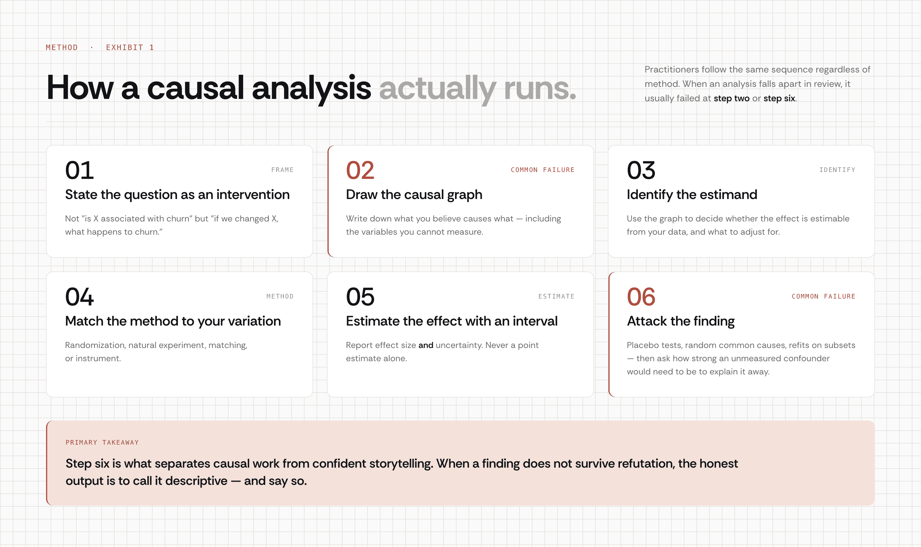
Step six is what separates causal work from confident storytelling. When a finding does not survive refutation, the honest output is to call it descriptive and say so.

Causal inference and machine learning

Machine learning optimizes prediction. Causal inference optimizes explanation. They are not competing, and confusing them is expensive.

A churn model that assigns an account a 73% probability of leaving is genuinely useful and completely silent on what to do. Its features are correlations, tuned for accuracy, and the strongest predictor is often a symptom rather than a cause. Cancellation-page visits predict churn beautifully. Preventing people from visiting that page prevents nothing.

Where the two fields meet is in estimation. Causal machine learning uses flexible models inside a causal framework: the model handles the nuisance work of adjusting for many covariates, while the causal design determines what is actually being estimated. Meta-learners and forest-based estimators extend this to conditional effects across subgroups.

Large language models are now part of this pipeline, though not in the way the marketing usually suggests. An LLM does not perform causal inference. What it does well is convert unstructured text into structured variables that a causal model can consume, turning a support transcript into typed fields that behave like any other column in a warehouse.

Where descriptive analytics stops

Most companies already own tools that report on customer data. Experience management platforms, BI dashboards, and text analytics suites all produce topic rankings and driver analyses, and they are useful for knowing that a problem exists.

The method underneath those driver analyses is almost always volume plus correlation with the score. That is a level-one answer wearing a level-two label. It cannot distinguish a cause from a coincidence, which is exactly how a front desk ends up as priority number two.

If your answers stop after the first row, you have a map of symptoms without a diagnosis.

Causal inference on the data most companies never analyze

Here is the part the textbooks skip. Nearly every published treatment of causal inference draws its examples from epidemiology, economics, or public policy, where the variables were collected as numbers from the start.

Business causes are rarely numbers. They are sentences. The reason a customer left is in a call transcript, a survey verbatim, or a chat log, and 80% to 90% of enterprise data is unstructured, while only 18% of organizations in a Deloitte survey reported being able to take advantage of it. Executives who count unstructured data among their most valuable sources are 24% more likely to have exceeded their business goals.

This is the real constraint on causal inference in business. Not the math, which is mature. The treatment variable does not exist in the warehouse yet.

Closing that gap requires turning language into structured, queryable fields at the record level, every record rather than a sample, then joining those fields to the metrics that quantify impact. Once "the customer reported a repeat transfer" is a typed column sitting next to ARR, tenure, and renewal date, it can be a treatment variable like any other. That layer is what Dimension Labs builds, we call it Causal Intelligence, and it is what makes causal estimates on customer conversations possible at all.

The output stops looking like a topic chart and starts looking like this:

Mid-market churn up 18% quarter over quarter. Primary driver: repeat transfers in support during the first 90 days. Supporting evidence: ATE +0.23 on churn probability, 95% CI [0.18, 0.28], p < 0.01, adjusted for plan type, tenure, and segment; effect concentrated in accounts under 90 days (CATE +0.34) and near zero in enterprise accounts past two years. Survives placebo and random-common-cause refutation. Recommended action: route first-90-day accounts to a dedicated queue. Exposure: 34 accounts, $4.7M ARR.

Key terms

Treatment. The variable whose effect you want to estimate. Outcome. The metric you expect the treatment to move. Confounder. A variable causing both treatment and outcome. Adjust for it. Collider. A variable caused by both. Do not adjust for it. Counterfactual. What would have happened under a different action. ATE / CATE. Average effect across a population, and within a subgroup. Backdoor criterion. The graph-based rule for which variables close confounding paths. Refutation test. A deliberate attempt to break your own finding before publishing it.

So what would change if your next quarterly review reported effect sizes and confidence intervals instead of topic counts? And how many initiatives currently on the roadmap were prioritized by mention volume?

Counting is not knowing. Causal inference is the difference.

Frequently Asked Questions

What is causal inference in simple terms?

Causal inference is the practice of estimating whether changing one thing would change another, and by how much. It goes beyond noticing that two variables move together by explicitly modeling what would have happened under a different action. The result is an effect size with a confidence interval, not a ranking of correlations.

How is causal inference different from predictive modeling?

Predictive models answer what will happen and are optimized for accuracy, so their strongest features are often symptoms rather than causes. Causal models answer what would happen if you intervened, which is the question behind any decision to spend money or change a process. A model can predict churn with high accuracy and still give you nothing to act on.

Can you do causal inference without running an experiment?

Yes, and most business causal inference is observational because the events already happened. Difference-in-differences, propensity score matching, instrumental variables, synthetic control, and double machine learning all construct a credible counterfactual from historical data. Each depends on assumptions that must be stated in advance and stress-tested afterward with placebo and refutation checks.

What is causal inference in LLMs?

Large language models do not perform causal inference on their own, since they generate text based on learned patterns rather than estimating effects under intervention. Their practical role is upstream: extracting structured variables from unstructured text so that transcripts, tickets, and verbatims can enter a causal model as typed fields. The causal work still happens in formal estimation libraries like DoWhy or EconML.

If you want to see what causal inference finds in your own customer conversations, book a demo with Dimension Labs.

Sources:

1. MIT Sloan Management, "Tapping the power of unstructured data." https://mitsloan.mit.edu/ideas-made-to-matter/tapping-power-unstructured-data

2. Deloitte Insights, "The insight-driven organization: Analytics and AI-driven enterprises thrive in the Age of With" (2019). https://www.deloitte.com/us/en/insights/topics/analytics/insight-driven-organization.html

3. Harvard Business Review, Ron Kohavi and Stefan Thomke, "The Surprising Power of Online Experiments" (2017). https://hbr.org/2017/09/the-surprising-power-of-online-experiments